From a Trading Bot to an AI Trading Arena
Building, testing, and revising a small-account trading experiment
Abstract
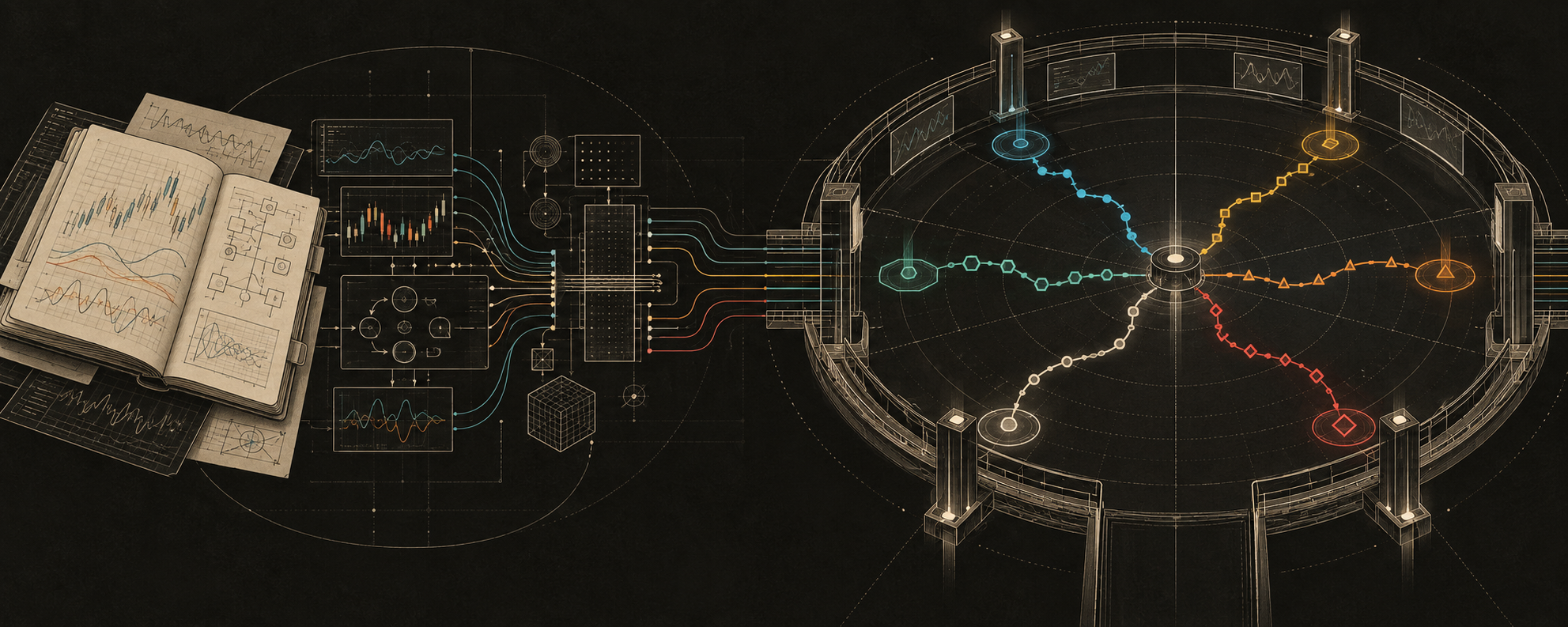
This project began with an intraday trading bot: quantitative indicators, a local language-model analyst, a skeptical review pass, a Gemini trade planner, and a Telegram interface. The idea was to turn market data into a more disciplined decision process. Testing exposed problems at several levels: inconsistent inputs, prompts that encouraged unnecessary trades, promising patterns that failed on another period, and transaction costs that overwhelmed the measured gross result. Those findings led to the AI Trading Arena, a framework that separates model decisions from simulated execution and compares them with explicit controls. In the recorded shared-period Arena test, six models and four controls each began with $100. All six models lost money after modeled costs; a capped SPY position finished first. This article traces that progression, explains what the experiments actually measured, and documents the changes planned before the next run.
1. The original question
I wanted to find out whether a structured AI workflow could make useful trading decisions for a small account.
The starting point was a specific strategy family: intraday momentum in stocks showing unusual price and volume activity. The bot would identify candidates, calculate technical context, investigate the setup, challenge the bullish case, and produce a trade plan with an entry, stop, and targets.
That architecture gave me several things I could inspect. There was code behind the indicators. There were prompts behind the recommendations. There was a journal behind the feedback loop. There were explicit prices behind the proposed trades.
The difficult part was determining whether any of those components improved the outcome.
A coherent explanation can make a trade feel justified. A well-organized pipeline can make that explanation feel tested. Neither tells me how the same process behaves across hundreds of opportunities after execution costs.
The project therefore developed along two tracks: building the decision system and building the means to challenge it. Eventually, the second track became the Arena.
Three different objects appear in this account: the original AI-assisted bot, historical tests of its mechanical trading rules, and the later Arena comparison. Keeping them distinct is essential. The original backtests did not establish the contribution of every model call in the live workflow, and the Arena changed both the decision interface and the trading clock.
All performance figures below come from historical simulations and saved project artifacts. They describe the tests that were run.
2. Inside the original bot
The original files contain a substantial trading workflow. The main components handled market data, quantitative calculations, model reasoning, trade-plan validation, monitoring, and journaling.
The analyst used a local Qwen model through Ollama. It could request additional information through a tool loop: the model requested a tool, Python executed it, and the result returned to the conversation. Available functions included ticker data, news, filings, and market context.
A separate devil’s-advocate pass challenged the setup. Gemini then served as a trade planner, combining the candidate analysis, risk review, and market data into a proposed trade or a decision to pass. Telegram provided the interface for reviewing the analysis, requesting the plan, and arming the monitor.
The journal added another layer. Recent trade history could be injected into later analysis, including instructions about conviction and drawdowns. That made the original design a stateful workflow: earlier activity could influence what the analyst was told next.
This was a useful software structure to investigate. It also created many possible explanations for a bad outcome. The candidate might have been weak. The data might have been stale. The analyst might have misunderstood it. The plan might have been late. The monitor might have entered at a price that no longer matched the plan.
Before judging the model, I needed to inspect that entire chain.
What the quantitative layer actually did
The quant_math.py module turned price and volume histories into a collection of market descriptors. Its calculations included:
- Momentum: RSI, stochastic RSI, rate of change, and CCI, describing recent movement and its position relative to recent history.
- Trend: MACD, exponential moving averages, and ADX with directional indicators, describing trend direction and strength.
- Volatility: ATR and Bollinger Bands, describing the size and distribution of recent price movement.
- Volume: relative volume, an OBV-based signal, and an approximate volume profile.
- A second time frame: a 15-minute indicator view alongside the main 5-minute calculations.
These features made the input more structured. They did not, by themselves, demonstrate a predictive advantage. Several are different transformations of the same underlying prices. Agreement among them cannot automatically be counted as independent evidence.
The implementation details mattered, too. The volume profile assigned a bar’s volume to the price bin containing its close. That is a useful approximation to describe the input, but it is not a reconstruction of every transaction at every price.
ATR connected the quantitative layer to trade geometry. In the revised plan, the intended distance from entry to stop was 1.5 times ATR. Calling that distance one risk unit, or R, the first and second targets were placed at 1.5R and 3R above entry.
For example, an entry at $10 with ATR of $0.20 produces a $0.30 risk distance: a $9.70 stop, a $10.45 first target, and a $10.90 second target. Those are planned levels before execution effects. They describe the payoff structure; the test still has to establish how often prices reach them and at what actual fills.
3. Correcting the inputs and the decision process
The first major review found problems that existed before a model could make a useful decision.
The indicators and the snapshot could describe different times
Some intraday requests used a timezone-naive local timestamp. The project review identified a five- to six-hour displacement when that timestamp was interpreted as UTC. The model could receive current snapshot prices alongside indicators calculated from much older bars.
That is a particularly misleading failure mode because each individual value can look plausible. The combined description is what fails: the price and the trend indicators no longer describe the same market state.
The correction used timezone-aware UTC requests. The indicator lookback was also extended so Monday calculations did not depend on finding enough data in a weekend-only interval.
Relative volume needed one definition
The pipeline had several incompatible relative-volume calculations. One compared cumulative volume with a linearly prorated full-day total. Another used the full previous day as its denominator. Premarket logic used another approximation.
As a result, the screener could rank a stock using one notion of unusual activity while the model was shown another.
The revised calculation compared cumulative volume with prior sessions at the same time of day when the data supported it. Conceptually:
Relative volume at time t = today’s cumulative volume through t / average prior-session cumulative volume through t.
That gave the feature a consistent meaning across the workflow. It still needed testing as a signal, but at least the different components could agree on what the number represented.
Passing had to be a valid outcome
Earlier prompts pushed the system toward taking a trade even when the setup was marginal. The review removed that pressure, reconciled conflicting stop instructions, and added a programmatic quality gate after the model’s response.
The gate checked minimum conviction, relative volume, and reward-to-risk requirements. Validation fallbacks rebuilt malformed stops and targets from ATR. The monitor also gained checks against entering too far above the planned price and logic to reanchor the plan to the entry fill.
These changes improved consistency. They did not settle the question of profitability. A correctly implemented rule can still select unprofitable trades.
4. What the original trials showed
The early tests produced exactly the kind of result that invites further tuning: an overall loss with an attractive pocket inside it.
The initial short baseline contained 68 trades and lost $11.05. Its opening-scan subset looked much better: 16 trades, $13.16 in gains, and a profit factor of 1.82.
Profit factor is total winning-trade P/L divided by the absolute total of losing-trade P/L. A value above one means aggregate gains exceeded aggregate losses in that sample.
Sixteen trades were enough to suggest a hypothesis. They were insufficient to establish a reliable opening-time advantage, especially when the candidate universe was a curated list of known movers.
The broader six-month test contained 401 trades and lost $175.63. The opening-scan subset now lost $62.76 across 134 trades. Changing the post-target trailing rule barely changed the overall outcome.
Another apparent opportunity emerged in a narrower gap band. It looked favorable in the period used to discover it, then failed in the separate July–December 2025 test: 351 trades, a $137.35 loss, and a profit factor of about 0.82.
The sequence is more informative than any isolated winning subset. A pattern appeared, a rule was proposed, and another sample did not support it.
Recorded mechanical backtests
Scroll the table sideways to see all columns
| Test | Historical period | Trades | Net trade P/L | Profit factor |
|---|---|---|---|---|
| Short baseline, curated universe | June 15–July 17, 2026 | 68 | −$11.05 | 0.88 |
| Broader six-month baseline | January 5–July 17, 2026 | 401 | −$175.63 | 0.83 |
| Gap-band validation | July–December 2025 | 351 | −$137.35 | 0.82 |
| Two-year market-entry test | July 2023–June 2025 | 1,520 | −$835.86 | 0.77 |
| Two-year pullback-entry test | July 2023–June 2025 | 1,179 | −$565.90 | 0.78 |
These dollar figures sum simulated trades using a $100-per-trade sizing setting, with integer share quantities. They are not returns from a single continuously funded $100 portfolio. The original backtester did not enforce the cash constraints needed to interpret them that way. The later Arena did track portfolio cash and positions.
The two-year tests compared market entries with a pullback variant that waited for a limit price below the scan price. The pullback version lost less, but it also executed fewer trades. Its recorded profit factor remained below one.
The broader tests were primarily evaluations of the mechanical rules. They did not isolate the added value of Qwen’s research, the skeptical review, or Gemini’s planning. I could conclude that the tested rule system had not established a profitable result under those assumptions. I could not assign that entire result to an individual model.
5. The audit changed the diagnosis
A separate review of the backtester and raw trade files decomposed the two-year market-entry result into trading performance before and after the modeled slippage.
The recorded net result was −$835.86. The audit’s reconstruction before those costs was approximately +$10.62. The difference was approximately $846.48.
Gross profit factor was about 1.003, compared with 0.771 net.
That placed the central problem in clearer terms. Over this test, the selected trades were close to aggregate break-even before the assumed execution costs. There was little measured gross surplus available to pay those costs.
The original model charged 0.3% per side. To see the scale, a roughly 0.6% round trip against a 3% stop distance consumes about 0.2R. Tight stops make a fixed percentage execution charge large relative to the amount being risked.
The audit also challenged the backtester itself. Candidate discovery used a current active-symbol list, excluding names that had disappeared. Candidate ranking incorporated the day’s high, which would not have been available at a morning scan. Daily and intraday prices could use inconsistent split adjustments. Slippage was also charged to limit fills in ways that penalized some configurations.
Those findings point in different directions. They make it inappropriate to treat a single number as a precise estimate of live performance. The audit’s more favorable treatment of limit fills improved the pullback profit factor to about 0.91, still below one in that reconstruction.
Some language in the original review was more absolute than I would use in a research account. A finite, imperfect backtest does not prove that every possible filter, exit rule, or future strategy must fail. The supported conclusion is narrower: these trials had not demonstrated a repeatable advantage large enough to survive the modeled costs.
That was sufficient reason to change how I was conducting the experiment.
6. Why I built the Arena
The original bot combined a human-selected strategy, indicator engineering, multiple model roles, tool use, and execution logic. Improving the whole system at once made attribution difficult.
The Arena gave the model a more explicit job: consume a defined market view and submit a structured decision. A separate engine handled the portfolio and the simulated fills. Controls supplied reference outcomes.
The workflow has two stages:
- Decision generation. A model receives historical market features and returns a saved JSON response containing its thesis and proposed orders.
- Execution replay. The engine processes those saved decisions against the historical price panel, applying portfolio rules, exits, and modeled costs.
This separation is useful because I can inspect or replay an existing decision without asking the model to produce a different answer. The website’s comparison uses saved decisions; rendering the report does not require a fresh round of model calls.
The Arena also moves from intraday scans to one decision per trading session after the close, with orders intended for the next session’s open. That changes the problem. The Arena is not a direct continuation of the original 5-minute backtest, and its legacy momentum control is a daily adaptation of the earlier rules.
Despite the Training Arena name, this stage evaluates existing models. It does not update their weights or demonstrate that they learned from the tournament.
What a model actually sees
The historical data panel spans 2016–2022 and includes thousands of symbols, including names that later delisted. The model receives a compact view sampled from that panel, rather than every row of market data.
The view uses nine groups: rising movers, falling movers, most active names, gappers, liquid core names, oversold names, overbought names, stocks near a 20-day high, and high-volatility names. A symbol can appear in multiple groups.
Rows provide features such as price, gap and daily change, recent returns, ATR, average dollar volume, relative volume, and RSI. There is also SPY context. The local caches used up to five rows per group; the archived Gemini cache used up to eight. That difference belongs in the comparison because the saved inputs were not identical across all six models.
Unlike the original bot, an Arena model cannot call a research toolkit during this decision. It is not shown its current portfolio, previous fills, or an accumulating trade journal. This tests decisions from a supplied market snapshot, rather than an analyst continually managing a known book.
The structured response allows up to three proposed long positions with weights and optional exit parameters. Valid empty orders represent a pass. A failed response is recorded separately. Neither automatically closes existing holdings; the replay’s exit rules continue to operate.
7. The recorded Arena test
The public comparison uses March 31–December 29, 2016, covering 191 trading sessions. This is the intersection of the saved decision date ranges for all ten participants. It was selected by coverage, not by the best-performing interval.
Some participants have longer caches. Their extra years are not silently added to this table. All ten rows below use the same shared period.
Each portfolio began with $100. The recorded configuration allowed fractional shares, long positions only, no leverage, at most five concurrent positions, and a maximum 34% weight in one name. A new position needed at least $5. Cash settlement was immediate in this simulation.
The engine modeled spreads, market impact, stop-related execution penalties, and regulatory fee presets. Those amounts are simulation assumptions, rather than fees collected from an actual brokerage account. A 20% daily-loss setting was present in configuration, but the replay did not enforce it as an effective trading brake. It should not be counted as protection delivered by this run.
The controls
The Arena included four controls with different purposes:
- Capped SPY buy-and-hold: a simple passive reference under this replay’s per-name cap. It invested roughly a third of the starting account and retained the rest as cash. This is not a fully invested SPY total-return benchmark; the price series also does not include dividend total return.
- Random selection: reproducible random picks weighted toward more liquid names, giving a reference for active trading without a directional thesis.
- Mean reversion: a mechanical alternative to momentum.
- Legacy momentum: the original gap-and-volume idea adapted to the Arena’s daily clock.
The controls share the execution framework, but their realized trade counts and exposures differ from those of the models. Random is therefore a useful baseline, not a perfectly matched experiment isolating stock-selection skill.
Results
The ten portfolios closed 1,102 trades in total. Final balances and maximum drawdowns were:
Scroll the table sideways to see all columns
| Method | Final balance | Net return | Closed trades | Maximum drawdown |
|---|---|---|---|---|
| Capped SPY buy-and-hold | $103.25 | +3.25% | 1 | 2.10% |
| Phi-4 Mini | $88.14 | −11.86% | 24 | 49.40% |
| Gemini 2.5 Flash, archived cache | $85.46 | −14.54% | 50 | 18.04% |
| Random | $82.14 | −17.86% | 167 | 23.53% |
| Mean reversion | $60.67 | −39.33% | 112 | 55.92% |
| Gemma 2 9B | $46.98 | −53.02% | 112 | 54.23% |
| Mistral 7B | $43.38 | −56.62% | 163 | 62.44% |
| Llama 3.1 8B | $29.03 | −70.97% | 178 | 71.26% |
| Legacy momentum | $21.31 | −78.69% | 187 | 78.93% |
| Qwen 2.5 7B | $13.34 | −86.66% | 108 | 88.39% |
Maximum drawdown measures the largest percentage decline from an earlier peak in daily account value, including open positions. Because starting equity was $100, the dollar gain or loss and percentage return happen to have the same numerical value here.
All six models finished below their starting balance. None beat capped SPY. Phi-4 Mini and the archived Gemini run finished above the random control, while the remaining four models finished below it.
Those are the results produced by this test. They describe this period, these saved decisions, and this implementation. They do not establish a universal ranking of the models.
8. Reading beyond the leaderboard
Finishing ahead of another loser is a limited result
Phi-4 Mini lost less than random and made far fewer trades. It also experienced a 49.40% maximum drawdown, despite ending down only 11.86%.
The final balance alone makes its path look considerably more comfortable than it was. The result supports reporting relative loss reduction in this run. It does not establish a stable, low-risk strategy.
Different exposure and turnover are part of the outcome. To attribute the difference specifically to superior selection, a future comparison should also match or explicitly analyze those quantities.
Operational failure can resemble restraint
Gemini had 152 failed sessions out of 191, approximately 79.6%, associated with quota errors in the archived cache. It produced orders on 38 sessions and one valid empty response.
That is materially different from deliberately choosing not to trade on 152 days. A portfolio receiving fewer new orders can avoid some losses without demonstrating that the model identified those losses in advance.
Gemma supplies another useful distinction: its cache contained 68 valid empty-order sessions without recorded errors. A pass, a failed request, and an order rejected by portfolio constraints need separate labels if the behavior is to be interpreted correctly.
Costs explain part of the damage
Mistral accumulated about $68 in modeled costs and ended down about $57. The random control accumulated about $31 in costs and ended down about $18. Cost drag was large enough to change the sign of their trade-level accounting results when added back.
Other models remained negative even after such an add-back. Qwen, for example, lost about $87 while incurring about $52 in modeled costs. Costs were a substantial contributor, but they did not explain the entire loss.
Adding recorded costs back is an accounting decomposition. It is not a new frictionless portfolio simulation. Lower costs could preserve equity, change later position sizes, and allow trades that the recorded portfolio could no longer afford.
A flat line does not establish good risk management
The website replay plots cumulative net realized P/L when trades close. It is not a daily equity curve. An open position can change value while the plotted line stays flat. The SPY line remains flat until its eventual sale for the same reason.
A flat tail can also reflect constraints. At a 34% per-name cap and a $5 minimum position, an account below roughly $14.71 cannot fund a new capped position. Qwen finished at $13.34. Its cache still contained orders throughout the shared period, so late inactivity should not be described as a learned decision to stand down.
9. What I would change next time
The next run should address known implementation issues and make the comparisons easier to interpret. The recorded run remains the record of what this version produced; corrections should create a new result alongside it.
Correct the replay’s order of events
A review found that morning position sizing could use the same session’s closing prices for existing holdings. Those closing prices were unavailable when the morning order was supposed to execute.
The defect was reproduced in a small synthetic case. With the opening prices and earlier decisions held constant, changing an existing holding’s later close from $10 to $20 changed a new purchase from approximately 3.40 to 4.56 shares at the same $10 opening price.
The daily replay also processes some later exits before opening entries. The correction needs to prevent cash or position slots released later in a session from funding an earlier purchase. Opening cost and liquidity inputs require the same timing review.
This work is logged for the next run. Its effect on the published balances and rankings has not been measured. The appropriate comparison is to fix the timing, replay the same saved decisions, and report the differences in trades, costs, returns, and drawdowns.
Make model inputs and service availability comparable
The next comparison should use the same prompt and market-view settings across participants, with those settings saved alongside the decisions. Gemini’s larger archived view and quota failures make it a different operational condition from the local runs.
Decision quality and service reliability should both be reported. Keeping them visible as separate measurements will make clear whether a quiet portfolio reflects a pass, an outage, or an execution constraint.
Measure the account path and define success in advance
Daily equity, gross exposure, turnover, rejected orders, and time spent in cash should accompany realized P/L. A future random baseline should include multiple declared seeds and, where practical, comparisons matched on exposure and trade frequency.
Cost sensitivity should use declared scenarios and actual replays. The passive references should identify their allocation and price-versus-total-return treatment. Success criteria should specify the benchmark, acceptable drawdown, and evaluation period before the results are inspected.
The project also contains an earlier July 25 Arena report with overlapping historical windows. That is a separate experiment, and its engine history includes documented fixes involving window-end trades, delistings, and price adjustments. Its window count should not be presented as hundreds of independent confirmations of this shared-period result.
Finally, I want genuinely new evaluation periods, including a forward paper test with decisions recorded before outcomes occur. Date-filtered inputs alone do not establish that a modern language model has never encountered information about a historical company or event. This project has not measured that possible source of contamination.
10. What the project has established so far
The original bot made the trading workflow inspectable. Its trials showed how quickly an appealing explanation could outrun the evidence: a strong opening subset disappeared in broader testing, a selected gap band failed another period, and a nearly flat gross result became a substantial net loss under the cost model.
The Arena made more of those comparisons explicit. It saved decisions, separated them from execution, tracked portfolios, and placed models next to controls. The recorded result was unfavorable for all six models after costs, with meaningful differences in turnover, drawdown, and operational reliability.
That gives me a concrete research agenda. I need to correct the replay timing, hold the evaluation conditions more consistently, and determine whether any model can produce repeatable gains over appropriate controls with an acceptable account path.
The value of the project so far is that its conclusions have become more specific as the testing improved. I can identify which inputs were inconsistent, which apparent patterns failed, where costs accumulated, and which questions remain unanswered.
The next version has to earn a stronger conclusion from another recorded test.
Project sources
This article draws on the project’s source code, saved trade CSVs, decision caches, audit notes, and website replay data. The supporting development repository is private; this is a project research account rather than a claim of independently replicated results.
- Original system:
quant_math.py,ai_engine.py,tools.py,main.py,telegram_handlers.py,trade_monitor.py, andjournal.py. - Original experiments and review:
PIPELINE_ANALYSIS.md,INDEPENDENT_AUDIT.md,backtest.py, and the baseline, validation, market-entry, and pullback trade CSVs. - Arena methodology:
arena/agents/llm_agent.py,arena/agents/controls.py, portfolio and cost modules, andarena/engine/replay.py. - Recorded comparison: saved decision caches and
assets/arena-replay.json, including configuration and source hashes. - Next-run correction:
ARENA_RERUN_FIXES.md.
The interactive companion is the AI Trading Arena report.